Fitted Values for iAR, CiAR, and BiAR Classes
fit.RdFitted Values for the provided data. This method is implemented for: 1. Irregular Autoregressive models (`iAR`) 2. Complex Irregular Autoregressive models (`CiAR`) 3. Bivariate Autoregressive models (`BiAR`)
Arguments
- x
An object of class
iAR,CiAR, orBiAR, containing the model specification and parameters:For
iAR:family: The distribution family of the iAR model (one of "norm", "t", or "gamma").series: A numeric vector representing the time series to be fitted.coef: The coefficient(s) of the iAR model.times: A numeric vector specifying the time points of the series.zero_mean: Logical, whether to fit a zero-mean model.standardized: Logical, whether the model output should be standardized (for "norm" family).mean: The mean parameter (only for "gamma" family).
For
CiAR:coef: The real and imaginary parts of the CiAR model's coefficients.series: A numeric vector representing the time series to be fitted.times: A numeric vector specifying the time points of the series.zero_mean: Logical, whether to fit a zero-mean model.standardized: Logical, whether the model output should be standardized.c: A scaling parameter for the CiAR model.
For
BiAR:coef: The coefficients of the BiAR model (real and imaginary parts).series: A numeric matrix with two columns representing the bivariate time series to be fitted.times: A numeric vector specifying the time points of the series.series_esd: A numeric matrix for the error structure (optional, used internally).zero_mean: Logical, whether to fit a zero-mean model.
- ...
Additional arguments (unused).
Value
An updated object of class iAR, CiAR, or BiAR, where the fitted_values property contains the fitted time series values.
Details
This method fits the specified time series model to the data contained in the object. Depending on the class of the input object:
For
iAR, the function supports three distribution families:"norm" for normal distribution.
"t" for t-distribution.
"gamma" for gamma distribution.
For
CiAR, the function uses complex autoregressive processes.For
BiAR, the function fits a bivariate autoregressive process.
All required parameters (e.g., coefficients, time points) must be set before calling this method.
References
Eyheramendy S, Elorrieta F, Palma W (2018). “An irregular discrete time series model to identify residuals with autocorrelation in astronomical light curves.” Monthly Notices of the Royal Astronomical Society, 481(4), 4311-4322. ISSN 0035-8711, doi:10.1093/mnras/sty2487 , https://academic.oup.com/mnras/article-pdf/481/4/4311/25906473/sty2487.pdf. ,Elorrieta, F, Eyheramendy, S, Palma, W (2019). “Discrete-time autoregressive model for unequally spaced time-series observations.” A&A, 627, A120. doi:10.1051/0004-6361/201935560 . ,Elorrieta F, Eyheramendy S, Palma W, Ojeda C (2021). “A novel bivariate autoregressive model for predicting and forecasting irregularly observed time series.” Monthly Notices of the Royal Astronomical Society, 505(1), 1105-1116. ISSN 0035-8711, doi:10.1093/mnras/stab1216 , https://academic.oup.com/mnras/article-pdf/505/1/1105/38391762/stab1216.pdf.
Examples
# Example 1: Fitting a normal iAR model
library(iAR)
n=100
set.seed(6714)
o=iAR::utilities()
o<-gentime(o, n=n)
times=o@times
model_norm <- iAR(family = "norm", times = times, coef = 0.9)
model_norm <- sim(model_norm)
model_norm <- kalman(model_norm)
model_norm <- fit(model_norm)
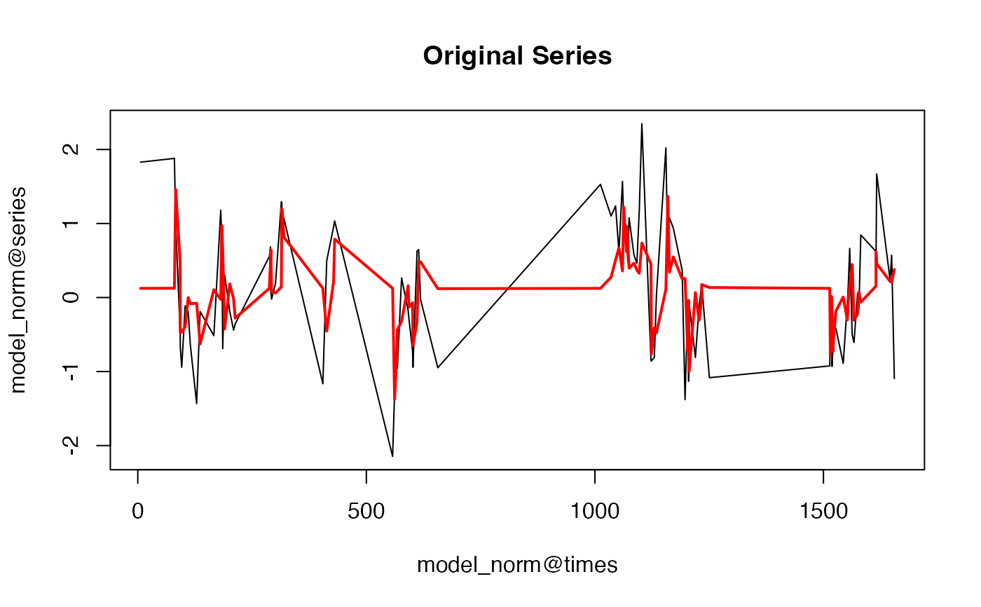
plot(model_norm@times, model_norm@series, type = "l", main = "Original Series")
lines(model_norm@times, model_norm@fitted_values, col = "red", lwd = 2)

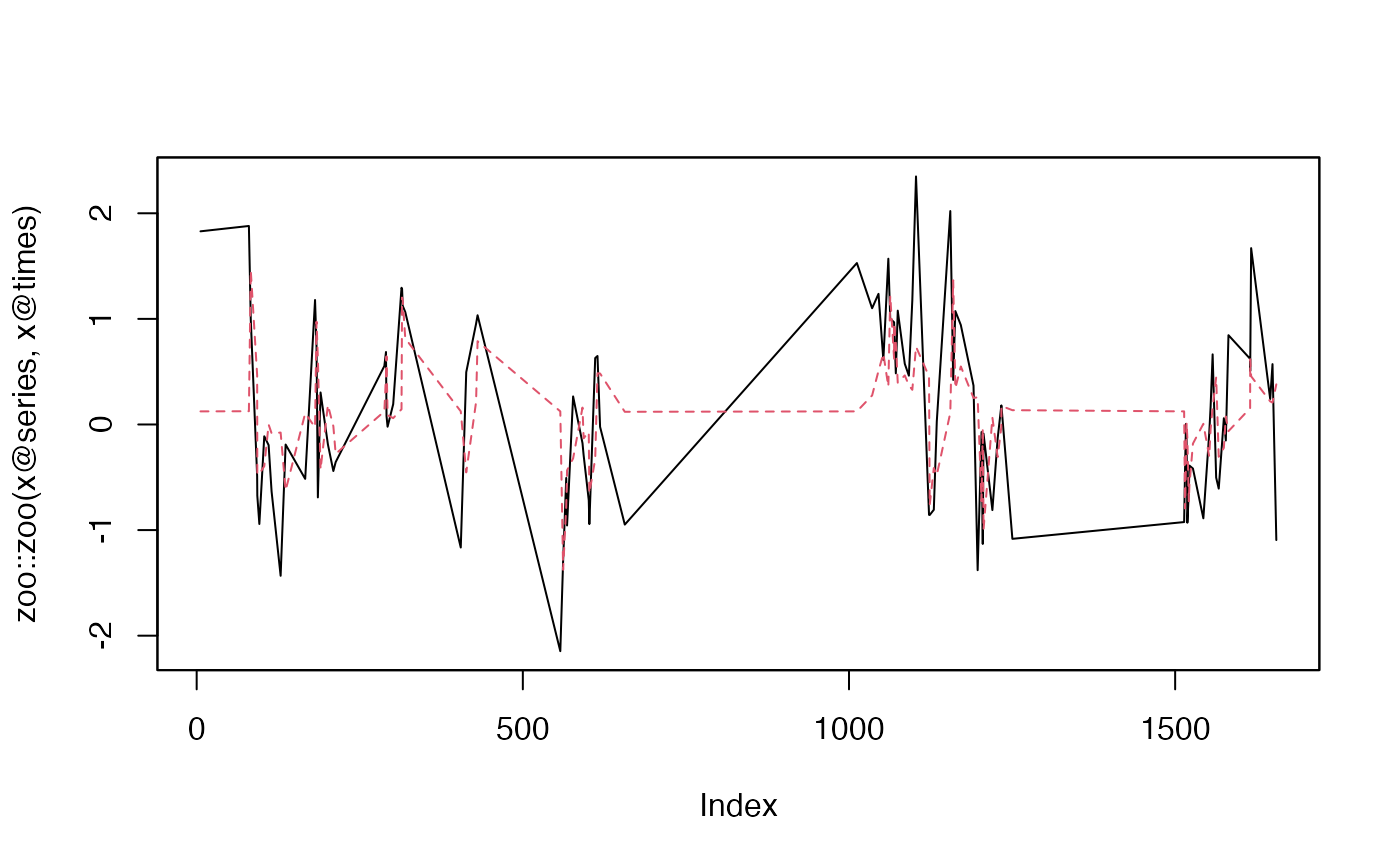
plot_fit(model_norm)


# Example 2: Fitting a CiAR model
set.seed(6714)
model_CiAR <- CiAR(times = times,coef = c(0.9, 0))
model_CiAR <- sim(model_CiAR)
y=model_CiAR@series
y1=y/sd(y)
model_CiAR@series=y1
model_CiAR@series_esd=rep(0,n)
model_CiAR <- kalman(model_CiAR)
print(model_CiAR@coef)
#> [1] 0.9199923 0.1072453
model_CiAR <- fit(model_CiAR)
yhat=model_CiAR@fitted_values

# Example 3: Fitting a BiAR model
n=80
set.seed(6714)
o=iAR::utilities()
o<-gentime(o, n=n)
times=o@times
model_BiAR <- BiAR(times = times,coef = c(0.9, 0.3), rho = 0.9)
model_BiAR <- sim(model_BiAR)
y=model_BiAR@series
y1=y/apply(y,2,sd)
model_BiAR@series=y1
model_BiAR@series_esd=matrix(0,n,2)
model_BiAR <- kalman(model_BiAR)
print(model_BiAR@coef)
#> [1] 0.9061971 0.3054558
model_BiAR <- fit(model_BiAR)
print(model_BiAR@rho)
#> [1] 0.8114818
yhat=model_BiAR@fitted_values